Atmospheric models (pycraf.atm)

Introduction

The atm sub-package can be used to calculate the atmospheric attenuation, which is relevant for various purposes. Examples would be to calculate the propagation loss associated with a terrestrial path, or a so-called slant path between a terminal at large height (e.g., a satellite) and an Earth terminal. The latter case is also of interest for observations of deep-space objects, as Earth’s atmosphere dampens the signal of interest. Especially, in astronomy one needs to correct for such attenuation effects to determine the original intensity of an object.

The relevant ITU-R Rec. P.676-11 contains two models. The Annex-1 model is more accurate and is valid for frequencies between 1 and 1000 GHz. It constructs the attenuation spectrum from the Debye continuum absorption and water and oxygen resonance lines. In contrast, Annex-2 is based on a simpler empirical method, that works for frequencies up to 350 GHz only. It doesn’t work with layers but assumes just a one-layer slab having an effective temperature, which would produce the same overall loss as the multi-layered model. Of course, this effective temperature has nothing to do with the true physical temperature (profile) of the atmosphere. Although the Annex-2 model is simpler and thus somewhat faster in principle, in most cases users of pycraf will want to use Annex-1 functions. These are mostly implemented in Cython and therefore reasonably fast.

Both Annexes provide a framework to calculate the specific attenuation (dB / km) for an atmospheric slab. To compute the full path loss caused by the atmosphere over a longer path, one has to integrate over the distance. For ground-to-ground stations this is trivial (assuming the specific attenuation is constant - which would not be true, if one station is at a significantly different altitude). For slant paths, Annex 1 and 2 methods differ substanially. 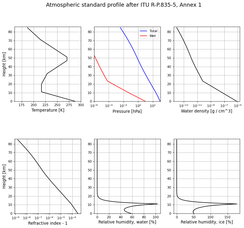The former determines the specific attenuation for potentially hundreds of different layers and as such height profiles for temperature and pressures are necessary. These are provided in ITU-R Rec. P.835-5. The atm sub- package contains the “Standard profile” (profile_standard) and five more specialized profiles, associated with the geographic latitude and season (profile_highlat_summer, profile_highlat_winter, profile_midlat_summer, profile_midlat_winter, and profile_lowlat).

Using pycraf.atm

Height profiles

Let’s start by having a look at the atmospheric standard height profile:

>>> import numpy as np
>>> import matplotlib.pyplot as plt
>>> from pycraf import atm
>>> from pycraf import conversions as cnv
>>> from astropy import units as u
>>>
>>> # define height grid
>>> height_grid = np.arange(0, 85, 0.1) * u.km
>>>
>>> # query profile_standard function
>>> hprof = atm.profile_standard(height_grid)
>>>
>>> # Plot various quantities
>>> _heights = height_grid.to(u.km).value
>>>
>>> plt.close()
>>> fig, axes = plt.subplots(2, 3, figsize=(12, 10))
>>> axes[0, 0].plot(hprof.temperature.to(u.K).value, _heights, 'k-')  
>>> axes[0, 0].set_xlabel('Temperature [K]')  
>>> axes[0, 0].set_xlim((160, 300))  
>>> axes[0, 1].plot(hprof.pressure.to(u.hPa).value, _heights, 'b-', label='Total')  
>>> axes[0, 1].plot(hprof.pressure_water.to(u.hPa).value, _heights, 'r-', label='Wet')  
>>> axes[0, 1].legend(
...     *axes[0, 1].get_legend_handles_labels(),
...     loc='upper right', fontsize=10
...     )  
>>> axes[0, 1].set_xlabel('Pressure [hPa]')  
>>> axes[0, 1].semilogx()  
>>> axes[0, 1].set_xlim((1.e-6, 1100))  
>>> axes[0, 2].plot(hprof.rho_water.to(u.g / u.cm ** 3).value, _heights, 'k-')  
>>> axes[0, 2].set_xlabel('Water density [g / cm^3]')  
>>> axes[0, 2].semilogx()  
>>> axes[1, 0].plot(hprof.ref_index.to(cnv.dimless).value - 1., _heights, 'k-')  
>>> axes[1, 0].set_xlabel('Refractive index - 1')  
>>> axes[1, 0].semilogx()  
>>> axes[1, 1].plot(hprof.humidity_water.to(u.percent).value, _heights, 'k-')  
>>> axes[1, 1].set_xlabel('Relative humidity, water [%]')  
>>> axes[1, 2].plot(hprof.humidity_ice.to(u.percent).value, _heights, 'k-')  
>>> axes[1, 2].set_xlabel('Relative humidity, ice [%]')  
>>> for idx, ax in enumerate(axes.flat):
...     ax.set_ylim((0, 86))  
...     if idx % 3 == 0:
...         ax.set_ylabel('Height [km]')  
...     ax.grid()  
...
>>> fig.suptitle(
...     'Atmospheric standard profile after ITU R-P.835-5, Annex 1',
...     fontsize=16
...     )  

(png, svg, pdf)

Here the function profile_standard returns a namedtuple with the plotted quantities. This works in the same way for the other special height profiles, provided in pycraf. Likewise, the user could define their own profiles, which will seamlessly work with all other functions in this package, as long as they use a compatible function signature (including return type) and extend to at least 85 km height.

Specific attenuation

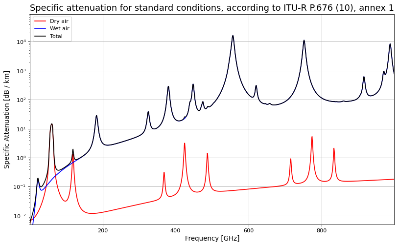
Given certain physical conditions such as temperature, pressure and water content, one can calculate the specific attenuation in the following manner. As the ITU-R Rec. P.676-11 methods work with the partial dry and wet air pressure, one usually has to derive these, e.g., from water content or humidity.

>>> _freqs = np.arange(1, 1000, 1)
>>> freq_grid = _freqs * u.GHz
>>> # weather parameter at ground-level
>>> total_pressure = 1013 * u.hPa
>>> temperature = 290 * u.K
>>> # water content is from the integral over the full height
>>> rho_water = 7.5 * u.g / u.m ** 3
>>>
>>> # alternatively, one can use atm.pressure_water_from_humidity
>>> pressure_water = atm.pressure_water_from_rho_water(temperature, rho_water)
>>> pressure_dry = total_pressure - pressure_water
>>>
>>> print(
...     'Oxygen pressure: {0.value:.2f} {0.unit}, '
...     'Water vapor partial pressure: {1.value:.2f} {1.unit}'.format(
...         pressure_dry, pressure_water
...     ))
Oxygen pressure: 1002.96 hPa, Water vapor partial pressure: 10.04 hPa
>>> atten_dry, atten_wet = atm.atten_specific_annex1(
...     freq_grid, pressure_dry, pressure_water, temperature
...     )
...
>>> plt.close()
>>> plt.figure(figsize=(12, 7))  
>>> plt.plot(
...     _freqs, atten_dry.to(cnv.dB / u.km).value,
...     'r-', label='Dry air'
...     )  
>>> plt.plot(
...     _freqs, atten_wet.to(cnv.dB / u.km).value,
...     'b-', label='Wet air'
...     )  
>>> plt.plot(
...     _freqs, (atten_dry + atten_wet).to(cnv.dB / u.km).value,
...     'k-', label='Total'
...     )  
>>> plt.semilogy()  
>>> plt.xlabel('Frequency [GHz]')  
>>> plt.ylabel('Specific Attenuation [dB / km]')  
>>> plt.xlim((1, 999))  
>>> plt.ylim((5.e-3, 0.9e5))  
>>> plt.grid()  
>>> plt.legend(*plt.gca().get_legend_handles_labels(), loc='upper left')  
>>> plt.title(
...     'Specific attenuation for standard conditions, '
...     'according to ITU-R P.676 (10), annex 1',
...     fontsize=16
...     )  

(png, svg, pdf)

Total attenuation

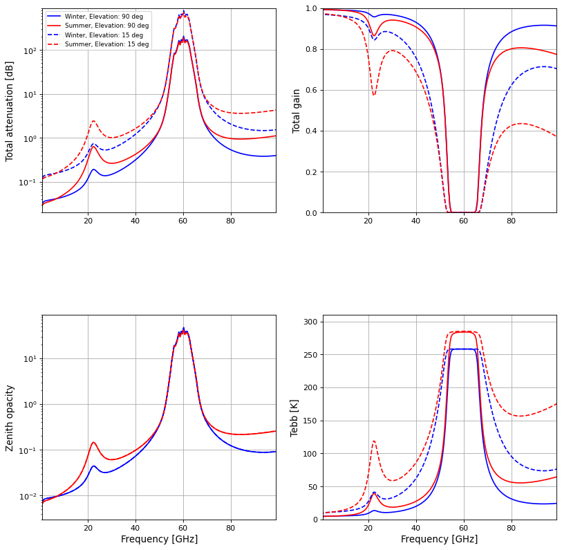
With the specific attenuation, one can infer the total attenuation along a terrestrial or slant path. For the latter scenario, one of course needs to calculate the specific attenuation for each atmospheric layer if working with Annex-1 formulas. If many calculations are to be done with the same atmospheric profile, the calculation of the physical parameters, including the frequency-dependent specific attenuation, would consume a lot of computing time. Therefore, atm Annex-1 functions use a dictionary to cache the height profiles. It has to be created once for a given atmospheric profile, by calling atm_layers, and can then be used for all subsequent calculations, e.g., by the atten_slant_annex1 function, which will do ray-tracing through the atmosphere and determine the overall atmospheric attenuation along the path.

Terrestrial path

For a terrestrial path, one only needs to multiply the specific attenuation, as inferred with atten_specific_annex1 and multiply with a distance:

>>> freqs = [1, 22, 30] * u.GHz
>>> total_pressure = 1013 * u.hPa
>>> temperature = 270 * u.K
>>> humidity = 80 * u.percent
>>>
>>> pressure_water = atm.pressure_water_from_humidity(
...     temperature, total_pressure, humidity
...     )
>>> pressure_dry = total_pressure - pressure_water
>>>
>>> print(
...     'Oxygen pressure: {0.value:.2f} {0.unit}, '
...     'Water vapor partial pressure: {1.value:.2f} {1.unit}'.format(
...         pressure_dry, pressure_water
...     ))
Oxygen pressure: 1009.11 hPa, Water vapor partial pressure: 3.89 hPa
>>> attens_dry, attens_wet = atm.atten_specific_annex1(
...     freqs, pressure_dry, pressure_water, temperature
...     )
>>> for freq, atten_dry, atten_wet in zip(freqs, attens_dry, attens_wet):
...     print('{:2.0f}: {:.3f} {:.3f}'.format(freq, atten_dry, atten_wet))
 1 GHz: 0.006 dB / km 0.000 dB / km
22 GHz: 0.016 dB / km 0.073 dB / km
30 GHz: 0.026 dB / km 0.034 dB / km
>>> distance = 10 * u.km
>>> attens_total = (attens_dry + attens_wet) * distance
>>> for freq, atten_total in zip(freqs, attens_total):
...     print('{:2.0f}: {:.3f}'.format(freq, atten_total))
 1 GHz: 0.063 dB
22 GHz: 0.887 dB
30 GHz: 0.598 dB

Slant path through layers of Earth’s atmosphere

For the slant path through the atmosphere, the user doesn’t need to provide the physical conditions manually, but one has to use one of the atmospheric height models, the properties of which are then cached via the atm_layers function.

>>> obs_alt = 300 * u.m
>>> _freqs = np.arange(0.25, 100, 0.5)
>>> freq_grid = _freqs * u.GHz
>>>
>>> cases = [
...     # elevation, profile, label, linestyle
...     (90 * u.deg, atm.profile_highlat_winter, 'Winter, Elevation: 90 deg', 'b-'),
...     (90 * u.deg, atm.profile_highlat_summer, 'Summer, Elevation: 90 deg', 'r-'),
...     (15 * u.deg, atm.profile_highlat_winter, 'Winter, Elevation: 15 deg', 'b--'),
...     (15 * u.deg, atm.profile_highlat_summer, 'Summer, Elevation: 15 deg', 'r--'),
...     ]
...
>>> plt.close()
>>> fig, axes = plt.subplots(2, 2, figsize=(12, 12))
>>> for elev, profile, label, linestyle in cases:
...
...     atm_layers_cache = atm.atm_layers(freq_grid, profile)
...     total_atten, refraction, tebb = atm.atten_slant_annex1(
...         elev, obs_alt, atm_layers_cache, t_bg=2.73 * u.K
...         )
...     opacity = atm.opacity_from_atten(total_atten, elev)
...
...     print('Refraction for {}: {:.1f}'.format(label, refraction.to(u.arcsec)))
...
...     _ = axes[0, 0].plot(_freqs, total_atten.to(cnv.dB).value, linestyle, label=label)
...     _ = axes[0, 1].plot(_freqs, 1 / total_atten.to(cnv.dimless).value, linestyle, label=label)
...     _ = axes[1, 0].plot(_freqs, opacity.to(cnv.dimless).value, linestyle, label=label)
...     _ = axes[1, 1].plot(_freqs, tebb.to(u.K).value, linestyle, label=label)
Refraction for Winter, Elevation: 90 deg: -0.0 arcsec
Refraction for Summer, Elevation: 90 deg: -0.0 arcsec
Refraction for Winter, Elevation: 15 deg: -228.6 arcsec
Refraction for Summer, Elevation: 15 deg: -237.9 arcsec
>>> axes[0, 0].semilogy()  
>>> axes[1, 0].semilogy()  
>>> axes[0, 0].legend(*axes[0, 0].get_legend_handles_labels(), loc='upper left', fontsize=8)  
>>> axes[0, 0].set_ylabel('Total attenuation [dB]')  
>>> axes[0, 1].set_ylabel('Total gain')  
>>> axes[1, 0].set_ylabel('Zenith opacity')  
>>> axes[1, 1].set_ylabel('Tebb [K]')  
>>> axes[0, 0].set_ylim((2e-2, 9e2))  
>>> axes[0, 1].set_ylim((0, 1))  
>>> axes[1, 0].set_ylim((3e-3, 9e1))  
>>> axes[1, 1].set_ylim((0, 310))  
>>>
>>> for idx, ax in enumerate(axes.flat):
...     ax.grid()  
...     ax.set_xlim((1, 99))  
...     if idx >= 2:
...         ax.set_xlabel('Frequency [GHz]')  
...

(png, svg, pdf)

Note

Note, to convert between total attenuation, \(\gamma\), and (zenith!) opacity, \(\tau\) (used in astronomy), use

\[ \begin{align}\begin{aligned}\gamma [\mathrm{dB}] = 10\log_{10} \gamma\\\gamma = 10^{\gamma [\mathrm{dB}] / 10}\\\gamma = e^{-\tau\cdot \mathrm{AM}},~ \mathrm{AM}\approx\frac{1}{\sin\delta}\\\tau = -\frac{1}{\mathrm{AM}}\ln\gamma\end{aligned}\end{align} \]

It is clear, the for very realistic results, one should work with an actual height profile valid for the day of observation, such as measured with a radio sonde for example.

Ray-tracing, refraction, and path-finding

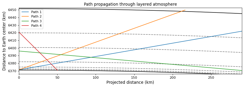
The function atten_slant_annex1, which was demonstrated above, internally calls a helper routine raytrace_path to work out the geometry of a path starting at a given altitude (above sea level) and with a certain elevation. As the refractive index of each atmospheric layer is slightly distinct, Snell’s law applies and bends the ray somewhat as it travels from layer to layer. The overall bending angle is called “refraction” and thus a source appears at a slightly different elevation angle for an observer.

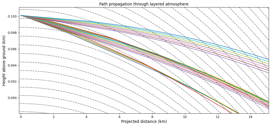
If you are interested in how such a path looks like, the following demonstrates how to plot it.

>>> # first, we need to create the atmospheric layer cache
>>> atm_layers_cache = atm.atm_layers([1] * u.GHz, atm.profile_highlat_winter)
>>>
>>> plt.close()
>>> fig = plt.figure(figsize=(12, 6))
>>>
>>> # to plot the atmospheric layers, we need to access the layers_cache:
>>> a_e = atm.EARTH_RADIUS
>>> layer_angles = np.arange(0, 0.1, 1e-3)
>>> layer_radii = atm_layers_cache['radii']
>>> bottom, top = layer_radii[[0, 900]]
>>> plt.plot(bottom * np.sin(layer_angles), bottom * np.cos(layer_angles), 'k-')  
>>> plt.plot(top * np.sin(layer_angles), top * np.cos(layer_angles), 'k-')  
>>> # we only plot some layers
>>> for r in layer_radii[[200, 500, 600, 700, 800, 850]]:
...     plt.plot(r * np.sin(layer_angles), r * np.cos(layer_angles), 'k--', alpha=0.5)  
...
>>> # now create four different example paths (of different type)
>>> for path_num, elevation, obs_alt, max_path_length in zip(
...         [1, 2, 3, 4],
...         [10, 20, -5, -45] * u.deg,
...         [300, 300, 25000, 50000] * u.m,
...         [1000, 230, 300, 1000] * u.km,
...         ):
...
...     path_params, _, refraction = atm.raytrace_path(
...         elevation, obs_alt, atm_layers_cache,
...         max_path_length=max_path_length,
...         )
...
...     print('total path length {:d}: {:5.1f}'.format(
...         path_num, np.sum(path_params.a_n)
...         ))
...
...     radii = path_params.r_n
...     angle = path_params.delta_n
...     x, y = radii * np.sin(angle), radii * np.cos(angle)
...     _ = plt.plot(x, y, '-', label='Path {:d}'.format(path_num))
total path length 1: 1000.0
total path length 2: 230.0
total path length 3: 300.0
total path length 4:  71.0
>>> plt.legend(*plt.gca().get_legend_handles_labels())  
>>> plt.xlim((0, 290))  
>>> plt.ylim((a_e - 5, 6453))  
>>> plt.title('Path propagation through layered atmosphere')  
>>> plt.xlabel('Projected distance (km)')  
>>> plt.ylabel('Distance to Earth center (km)')  
>>> plt.gca().set_aspect('equal')  

(png, svg, pdf)

As you can see, raytrace_path allows to specify a maximal path length (as well as a maximal separation angle, see API docs). This can be useful for terrestrial paths.

Note

The ITU-R Rec. P.676-11 only presents an algorithm for paths with an elevation angle larger than zero degrees. For pycraf the method was extended to work properly with negative elevation angles, as well.

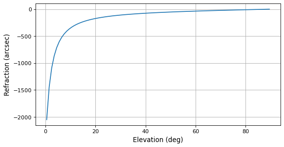
A similar function exists, path_endpoint, which only returns the parameters of the final point on the ray. For example, one could plot the refraction angle as a function of elevation:

>>> elevations = np.arange(0.5, 90, 1)
>>> obs_alt = 100 * u.m
>>> refractions = np.array([
...     atm.path_endpoint(
...         elev * u.deg, obs_alt, atm_layers_cache,
...         ).refraction.to(u.arcsec).value
...     for elev in elevations
...     ])
...
>>> plt.close()  
>>> fig = plt.figure(figsize=(8, 4))  
>>> plt.plot(elevations, refractions, '-')  
>>> plt.xlabel('Elevation (deg)')  
>>> plt.ylabel('Refraction (arcsec)')  
>>> plt.grid()  

(png, svg, pdf)

The function path_endpoint is really useful, because it allows us to find the correct elevation angle to have the path hit a certain point (e.g., a receiver station).

Caustics

Warning

Unfortunately, a model of atmospheric layers with discrete refractive indices leads to some unexpected effects. See the following.

Consider a situation, where multiple rays with slightly different elevation angles are computed:

>>> obs_alt = 0.1001 * u.km
>>> e_a = atm.EARTH_RADIUS
>>>
>>> layer_angles = np.linspace(-0.001, 0.02, 400)
>>> radii = atm_layers_cache['radii']
>>>
>>> plt.close()
>>> fig = plt.figure(figsize=(14, 6))
>>> for r in radii:
...     plt.plot(
...         r * np.sin(layer_angles),
...         r * np.cos(layer_angles) - e_a,
...         'k--', alpha=0.5
...         )  
...
>>> for elev in np.linspace(-0.04, -0.01, 21):
...     path_params, _, _ = atm.raytrace_path(
...         elev * u.deg, obs_alt, atm_layers_cache,
...         max_path_length=20 * u.km,
...         )
...     plt.plot(path_params.x_n, path_params.y_n - e_a, '-')  
...
>>> plt.xlim((-0.1, 15.1))  
>>> plt.ylim((obs_alt.value - 0.012, obs_alt.value + 0.001))  
>>> plt.title('Path propagation through layered atmosphere')  
>>> plt.xlabel('Projected distance (km)')  
>>> plt.ylabel('Height above ground (km)')  

(png, svg, pdf)

Depending on where exactly the paths hit the boundary of the next layer, a “split” of adjacent rays can occur. These “caustics” have drastic consequences: it is not possible to reach certain points in the atmosphere from a given starting point. This also makes it impossible to use non-stochastic optimization algorithms to find the optimal elevation angle to use for a transmitter-receiver link.

Finding the path to a given target

Pycraf comes with a utility function find_elevation that uses Basinhopping to find a good (not necessarily best) solution in the non-continuous minimization function (caused by the caustics, see above). This, unfortunately, can be relatively slow depending on path length and properties. It works by specifying the start and end height (above sea level) of the path and the true geographical angular distance between the two (see also true_angular_distance function):

>>> from pycraf.geometry import true_angular_distance
>>> lon_tx, lat_tx, h_tx = 6 * u.deg, 50 * u.deg, 30 * u.m
>>> lon_rx, lat_rx, h_rx = 6.03 * u.deg, 50.04 * u.deg, 2 * u.m
>>>
>>> arc_len = true_angular_distance(lon_tx, lat_tx, lon_rx, lat_rx)
>>> print('arc length: {:.4f}'.format(arc_len))
arc length: 0.0444 deg
>>> elev_opt, h_rx_opt = atm.find_elevation(
...     h_tx, h_rx, arc_len, atm_layers_cache
...     )
>>> print('Solution: elev = {:.3f} h_rx: {:.1f}'.format(
...     elev_opt, h_rx_opt.to(u.m)
...     ))
Solution: elev = -0.342 deg h_rx: 2.0 m

Note

A Jupyter tutorial notebook about the atm package is provided in the pycraf repository on GitHub. It also contains plots of the specialized height profiles, as well as an example for the Annex-2 method.

See Also

• Astropy Units and Quantities package, which is used extensively in pycraf.

• ITU-R Rec. P.453-12

• ITU-R Rec. P.835-5

• ITU-R Rec. P.676-11

Reference/API

pycraf.atm Package

The atm subpackage provides an implementation of the atmospheric models of ITU-R Rec. P.676-11. For this, various other algorithms from the following two ITU-R Recommendations are necessary:

• ITU-R Rec. P.835-5, which contains the Standard and several special atmospheric profiles.

• ITU-R Rec. P.453-12, which is used to calculate the refractive index from temperature and water/total air pressure. Furthermore, P.453 has formulae to derive the saturation water pressure from temperature and total air pressure, as well as the water pressure from temperature, pressure and humidity, or alternatively from temperature and wator vapor density.

Notes

The new version of P.676, ITU-R Rec. P.676-11, has updated the algorithms for Annex 2 (compare with https://www.itu.int/rec/R-REC-P.676-11-201609-I/en>). As the Annex 1 methods are more accurate (and sufficiently fast), users should use these for their work. pycraf continues to provide the Annex 2 solutions of the P.676-10 for historical reasons, but this should be considered as deprecated.

Functions

airmass_from_elevation(elev)	Airmass derived from elevation using extrapolation by Maddalena & Johnson.
atm_layers(freq_grid, profile_func[, heights])	Calculate physical parameters for atmospheric layers to be used with atten_slant_annex1 and other functions of the atm sub-package.
atten_from_opacity(tau[, elev])	Atmospheric attenuation derived from opacity.
atten_slant_annex1(elevation, obs_alt, ...)	Path attenuation for a slant path through full atmosphere according to ITU-R P.676-11 Eq (17-20).
atten_slant_annex2(atten_dry, atten_wet, ...)	Simple path attenuation for slant path through full atmosphere according to ITU-R P.676-10, Eq (28).
atten_specific_annex1(freq_grid, press_dry, ...)	Specific (one layer) atmospheric attenuation according to ITU-R P.676-11, Annex 1.
atten_specific_annex2(freq_grid, press, ...)	Specific (one layer) atmospheric attenuation based on a simplified algorithm according to ITU-R P.676-10, Annex 2.1.
atten_terrestrial(specific_atten, path_length)	Total path attenuation for a path close to the ground (i.e., one layer), according to ITU-R P.676-11, Annex 1 + 2.
elevation_from_airmass(airmass)	Airmass derived from elevation using extrapolation by Maddalena & Johnson.
equivalent_height_dry(freq_grid, press)	Equivalent height for dry air according to ITU-R P.676-10, Annex 2.2.
equivalent_height_wet(freq_grid, press)	Equivalent height for wet air according to ITU-R P.676-10, Annex 2.2.
find_elevation(obs_alt, target_alt, ...[, ...])	Finds the optimal path elevation angle from an observer to reach target.
humidity_from_pressure_water(temp, press, ...)	Relative humidity according to ITU-R P.453-12.
opacity_from_atten(atten[, elev])	Atmospheric opacity derived from attenuation.
path_endpoint(elevation, obs_alt, ...[, ...])	Calculate endpoint of propagation path through atmosphere by ray-tracing.
pressure_water_from_humidity(temp, press, ...)	Water pressure according to ITU-R P.453-12.
pressure_water_from_rho_water(temp, rho_w)	Water pressure according to ITU-R P.453-12.
profile_highlat_summer(height)	High latitude summer height profiles according to ITU-R P.835-5.
profile_highlat_winter(height)	High latitude winter height profiles according to ITU-R P.835-5.
profile_lowlat(height)	Low latitude height profiles according to ITU-R P.835-5.
profile_midlat_summer(height)	Mid latitude summer height profiles according to ITU-R P.835-5.
profile_midlat_winter(height)	Mid latitude winter height profiles according to ITU-R P.835-5.
profile_standard(height)	Standard height profiles according to ITU-R P.835-5, Annex 1.
raytrace_path(elevation, obs_alt, ...[, ...])	Calculate the propagation path geometry through atmosphere by ray-tracing.
refractive_index(temp, press, press_w)	Refractive index according to ITU-R P.453-12.
rho_water_from_pressure_water(temp, press_w)	Water density according to ITU-R P.453-12.
saturation_water_pressure(temp, press[, ...])	Saturation water pressure according to ITU-R P.453-12.