Antenna patterns (pycraf.antenna)#
Introduction#
In the antenna sub-package several antenna patterns are defined for
use in compatibility studies. These are merely toy models, but for such
studies they are usually sufficient.
Using pycraf.antenna#
Antenna patterns for fixed and mobile service (ITU-R Rec. F.1336)#
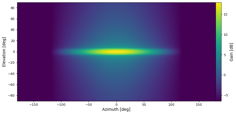
For fixed link and mobile communications (IMT), several antenna patterns are provided in ITU-R Rec F.1336-5.
Below, you can find a typical use case:
import numpy as np
import matplotlib.pyplot as plt
import pycraf.conversions as cnv
from pycraf.antenna import *
from astropy import units as u

azims = np.arange(-180, 180.1, 0.5) * u.deg
elevs = np.arange(-90, 90.1, 0.5) * u.deg

G0 = 18. * cnv.dB
phi_3db = 65. * u.deg
# theta_3db can be inferred in the following way:
theta_3db = 31000 / G0.to(cnv.dimless) / phi_3db.value * u.deg
k_p, k_h, k_v = (0.7, 0.7, 0.3) * cnv.dimless
tilt_m, tilt_e = (0, 0) * u.deg

bs_gains = imt_advanced_sectoral_peak_sidelobe_pattern_400_to_6000_mhz(
    azims[np.newaxis], elevs[:, np.newaxis],
    G0, phi_3db, theta_3db,
    k_p, k_h, k_v,
    tilt_m=tilt_m, tilt_e=tilt_e,
    ).to(cnv.dB).value

fig = plt.figure(figsize=(12, 6))
ax = fig.add_axes((0.15, 0.1, 0.7, 0.7))
cax = fig.add_axes((0.85, 0.1, 0.02, 0.7))

im = ax.imshow(
    bs_gains,
    extent=(azims[0].value, azims[-1].value, elevs[0].value, elevs[-1].value),
    origin='lower', cmap='viridis',
    )
plt.colorbar(im, cax=cax)
cax.set_ylabel('Gain [dB]')
ax.set_xlabel('Azimuth [deg]')
ax.set_ylabel('Elevation [deg]')
plt.show()
Feel free to play with the mechanical (tilt_m) and electrical (tilt_e)
tilt angles.
Note
At the moment only the sectoral peak- and average side lobe pattern for the frequency range between 400 MHz and 6 GHz are provided. This is the one, which can be used for IMT-advanced (LTE) basestations. Other patterns will follow.
WRC-19 Agenda Item 1.13, IMT2020#
For WRC-19 AI 1.13 ITU Study Group 3 (SG3) proposed to use a special newly
developed antenna pattern, which takes into account the phased array feeds of
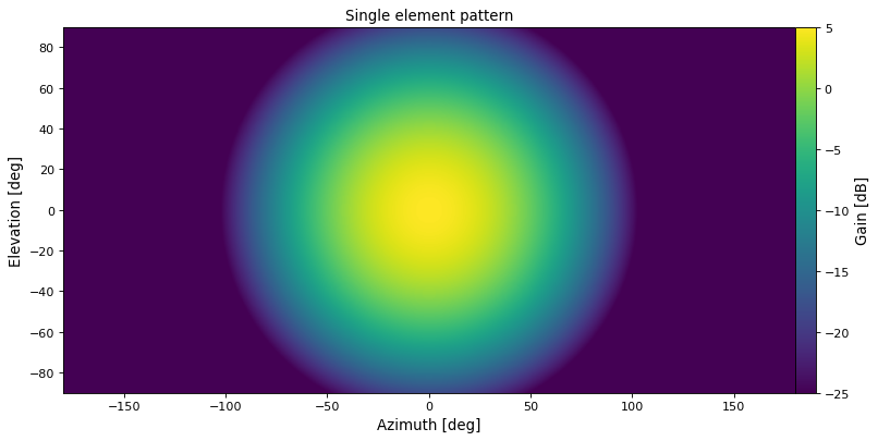
upcoming 5G devices. In pycraf, we provide a single-element pattern
(imt2020_single_element_pattern) - which can be useful for
generic compatibility studies in the spurious/out-of-band domain - and the
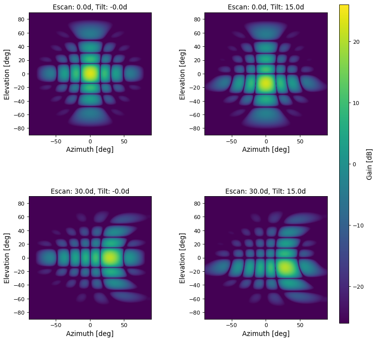
composite (aka phased-up) pattern,
imt2020_composite_pattern.
Both are easy to use. For example, plotting the patterns for base stations (with 8 x 8 elements):
import numpy as np
import matplotlib.pyplot as plt
import pycraf.conversions as cnv
from pycraf.antenna import *
from astropy import units as u

azims = np.arange(-180, 180.1, 0.5) * u.deg
elevs = np.arange(-90, 90.1, 0.5) * u.deg

# BS (outdoor) according to IMT.PARAMETER table 10 (multipage!)
G_Emax = 5 * cnv.dB
A_m, SLA_nu = 30. * cnv.dB, 30. * cnv.dB
azim_3db, elev_3db = 65. * u.deg, 65. * u.deg

gains_single = imt2020_single_element_pattern(
    azims[np.newaxis], elevs[:, np.newaxis],
    G_Emax,
    A_m, SLA_nu,
    azim_3db, elev_3db
    ).to(cnv.dB).value

fig = plt.figure(figsize=(12, 6))
ax = fig.add_axes((0.15, 0.1, 0.7, 0.7))
cax = fig.add_axes((0.85, 0.1, 0.02, 0.7))

im = ax.imshow(
    gains_single,
    extent=(azims[0].value, azims[-1].value, elevs[0].value, elevs[-1].value),
    vmin=-25, vmax=np.max(np.ceil(gains_single)),
    origin='lower', cmap='viridis',
    )
plt.colorbar(im, cax=cax)
cax.set_ylabel('Gain [dB]')
ax.set_xlabel('Azimuth [deg]')
ax.set_ylabel('Elevation [deg]')
ax.set_title('Single element pattern')
plt.show()

d_H, d_V = 0.5 * cnv.dimless, 0.5 * cnv.dimless
N_H, N_V = 8, 8

fig, axes = plt.subplots(2, 2, figsize=(12, 10))
fig.subplots_adjust(right=0.8)
cax = fig.add_axes([0.8, 0.1, 0.02, 0.8])

for i, azim_i in enumerate(u.Quantity([0, 30], u.deg)):
    for j, elev_j in enumerate(u.Quantity([0, -15], u.deg)):

        ax = axes[i, j]
        gains_array = imt2020_composite_pattern(
            azims[np.newaxis], elevs[:, np.newaxis],
            azim_i, elev_j,
            G_Emax,
            A_m, SLA_nu,
            azim_3db, elev_3db,
            d_H, d_V,
            N_H, N_V,
            ).to(cnv.dB).value

        gains_array[gains_array < -100] = -100  # fix blanks (-infty)
        im = ax.imshow(
            gains_array, extent=(
                azims[0].value, azims[-1].value,
                elevs[0].value, elevs[-1].value
                ),
            vmin=-26, vmax=26,
            origin='lower', cmap='viridis',
            )
        plt.colorbar(im, cax=cax)
        cax.set_ylabel('Gain [dB]')
        ax.set_xlabel('Azimuth [deg]')
        ax.set_ylabel('Elevation [deg]')
        ax.set_xlim((-90, 90))
        ax.set_ylim((-90, 90))
        ax.set_title(
            'Escan: {:.1f}d, Tilt: {:.1f}d'.format(
                azim_i.value, -elev_j.value
            ))
plt.show()
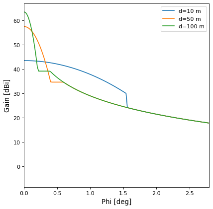
RAS telescope pattern#
This is a very simple approximation to the true pattern of a radio telescope, which neglects a lot of details such as blocking by feed support legs and cabin, stray cones, possible coma effects, and tapering functions.
Nevertheless, for most purposes in compatibility studies it should suffice. As an example, we plot the pattern:
import numpy as np
import matplotlib.pyplot as plt
from pycraf.antenna import ras_pattern
import astropy.units as u


phi = np.linspace(0, 20, 1000) * u.deg
diam = np.array([10, 50, 100]) * u.m
gain = ras_pattern(phi, diam[:, np.newaxis], 0.21 * u.m)
plt.plot(phi, gain.T, '-')
plt.legend(['d=10 m', 'd=50 m', 'd=100 m'])
plt.xlim((0, 2.8))
plt.xlabel('Phi [deg]')
plt.ylabel('Gain [dBi]')
plt.show()
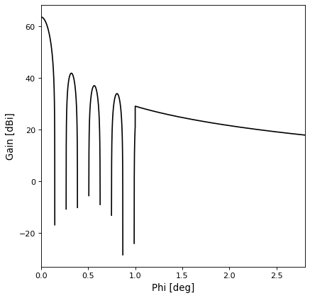
# zoom-in with Bessel correction
phi = np.linspace(0, 2.8, 10000) * u.deg
gain = ras_pattern(phi, 100 * u.m, 0.21 * u.m, do_bessel=True)
plt.plot(phi, gain, 'k-')
plt.xlim((0, 2.8))
plt.xlabel('Phi [deg]')
plt.ylabel('Gain [dBi]')
plt.show()

Fixed-links pattern#
Very similar to the RAS pattern, the fixed link pattern(s) work as follows:
import numpy as np
import matplotlib.pyplot as plt
from pycraf.antenna import *
from astropy import units as u

phi = np.linspace(0, 21, 1000) * u.deg
diam = np.array([1, 2, 10])[:, np.newaxis] * u.m
wavlen = 0.03 * u.m  # about 10 GHz
G_max = fl_G_max_from_size(diam, wavlen)
gain = fl_pattern(phi, diam, wavlen, G_max)

plt.plot(phi, gain.T, '-')
plt.legend(['d=1 m', 'd=2 m', 'd=10 m'])
plt.xlim((0, 21))
plt.xlabel('Phi [deg]')
plt.ylabel('Gain [dBi]')
plt.show()
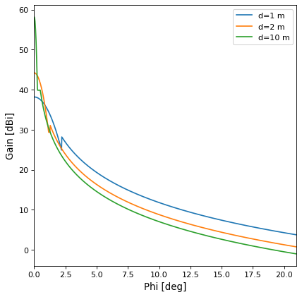
Note
There are different fixed-link patterns defined in ITU-R Rec. F.699-7, depending on the frequency and diameter-over-wavelength ratio.
See Also#
Astropy Units and Quantities package, which is used extensively in pycraf.
Reference/API#
pycraf.antenna Package#
This sub-package provides various (simplified) antenna patterns for use in compatibility studies. At the moment, the following are implemented:
IMT phased array antenna patterns for base station and mobile devices to be used for AI 1.13 IMT2020 studies. These are defined in the so-called IMT.MODEL document (ITU-R TG 5/1 document 5-1/36).
A pattern that can be used for radio telescopes (ITU-R Rec. RA.1631-0).
Pattern for fixed wireless systems (“fixed-links”), as defined in ITU-R Rec. F.699-7.
Functions#
|
Estimate maximum gain from antenna hpbw after ITU-R Rec F.699. |
|
|
|
|
|
|
|
Composite (array) antenna pattern according to `Rec. |
|
Extended composite (array) antenna pattern according to R19-WP5D-C-0716 document, which is an extension of the composite pattern introduced in `Rec. |
|
Single antenna element's pattern according to IMT.MODEL document. |
|
|
|
|
|
Antenna gain as a function of angular distance after ITU-R Rec RA.1631. |