Path attenuation, terrain data, and geodesics (pycraf.pathprof)#
Introduction#
The pathprof subpackage is probably the most important piece of
pycraf. It offers tools to calculate so-call path attenuation (propagation
loss), which is a key ingredient for compatibility studies in Radio spectrum
management. All kinds of Radio services have to cooperate and do their best to
not harm other users/services of the spectrum - neither in the allocated
spectral band, nor in the out-of-band or spurious domain (aka spectral
sidelobes). For this, it is fundamental to calculate the propagation loss that
a transmitted signal will experience before it is entering the receiving
terminal system.
There are a lot of parameters and environmental conditions that determine the propagation loss, such as the frequency, \(f\), of radiation, the distance, \(d\), between transmitter and receiver, the antenna gains and boresight angles, but also the terrain along the propagating path. For close distances, one often has the line-of-sight case, where the path loss is approximately proportional to \(d^{-2}f^{-2}\) (numbers smaller than One, mean an attenuation), i.e., the loss quickly gets larger with distance and frequency. For longer separations, other effects start to play a more important role:
Tropospheric scatter loss
Ducting and anomalous layer refraction loss
Diffraction loss
Clutter loss
Especially, for diffraction loss, information on the terrain heights is
needed. Therefore, pycraf implements functions to query
SRTM data, which was obtained from
a space shuttle mission. SRTM data has high spatial resolution of 3” (90 m),
which makes it more than appropriate for path propagation calculations.
In order to calculate the overall path attenuation, pycraf follows the algorithm proposed in ITU-R Recommendation P.452. We refer the user to this document to learn more about the details of such calculations, because the matter is quite complex and beyond the scope of this user manual.
Several helper routines are necessary to collect the necessary parameters for the P.452 calculations, that fall in the following categories:
Height profile (terrain map) construction.
Determination of Geodesics (the Great-circle path equivalent on the Earth’s ellipsoid, the so-called Geoid).
Finding radiometerological data for the path’s midpoint, which is also necessary to determine the effective Earth radii.
Note
For most of the functionality in this module, you will need to download SRTM tile data; see Working with SRTM data.
Getting Started#
Height profiles#
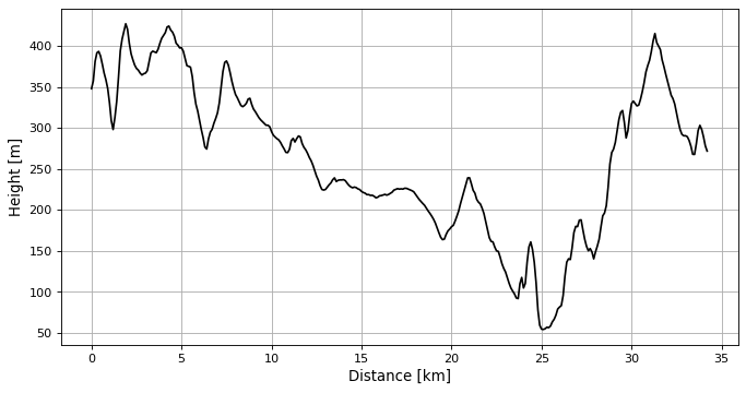
Let’s start with querying SRTM data and plot a height profile.
import matplotlib.pyplot as plt
from pycraf import pathprof
from astropy import units as u

# allow download of missing SRTM data:
pathprof.SrtmConf.set(download='missing')

lon_t, lat_t = 6.8836 * u.deg, 50.525 * u.deg
lon_r, lat_r = 7.3334 * u.deg, 50.635 * u.deg
hprof_step = 100 * u.m

(
    lons, lats, distance,
    distances, heights,
    bearing, back_bearing, back_bearings
    ) = pathprof.srtm_height_profile(
        lon_t, lat_t, lon_r, lat_r, hprof_step
        )

_distances = distances.to(u.km).value
_heights = heights.to(u.m).value

plt.figure(figsize=(10, 5))
plt.plot(_distances, _heights, 'k-')
plt.xlabel('Distance [km]')
plt.ylabel('Height [m]')
plt.grid()

Note
If the profile resolution, hprof_step is made large,
Gaussian smoothing is applied to avoid aliasing effects.
Path attenuation#
The pathprof package implements ITU-R Recommendation P.452-16 for path propagation
loss calculations. In pathprof this is a two-step procedure.
First a helper object, a PathProp object, has to be
instantiated. It contains all kinds of parameters that define the path
geometry and hold other necessary quantities (there are many!). Second, one
feeds this object into one of the functions that calculate attenuation
Line-of-sight (LoS) or free-space loss:
loss_freespaceTropospheric scatter loss:
loss_troposcatterDucting and anomalous layer refraction loss:
loss_ductingDiffraction loss:
loss_diffraction
Of course, there is also a function (loss_complete) to
calculate the total loss (a non-trivial combination of the above). As the
pathprof.complete_loss function also returns the most important constituents,
it is usually sufficient to use that. The individual functions are only
provided for reasons of computing speed, if one is really only interested in
one component:
>>> from pycraf import pathprof, conversions as cnv
>>> from astropy import units as u

>>> pathprof.SrtmConf.set(download='missing')

>>> freq = 1. * u.GHz

>>> lon_tx, lat_tx = 6.8836 * u.deg, 50.525 * u.deg
>>> lon_rx, lat_rx = 7.3334 * u.deg, 50.635 * u.deg
>>> hprof_step = 100 * u.m  # resolution of height profile

>>> omega = 0. * u.percent  # fraction of path over sea
>>> temperature = 290. * u.K
>>> pressure = 1013. * u.hPa
>>> time_percent = 2 * u.percent  # see P.452 for explanation
>>> h_tg, h_rg = 5 * u.m, 50 * u.m
>>> G_t, G_r = 0 * cnv.dBi, 15 * cnv.dBi

# clutter zones
>>> zone_t, zone_r = pathprof.CLUTTER.URBAN, pathprof.CLUTTER.SUBURBAN

>>> pprop = pathprof.PathProp(
...     freq,
...     temperature, pressure,
...     lon_tx, lat_tx,
...     lon_rx, lat_rx,
...     h_tg, h_rg,
...     hprof_step,
...     time_percent,
...     zone_t=zone_t, zone_r=zone_r,
...     )
The PathProp object is immutable, so if you want to change something, you have to create a new instance. This is, because, many member attributes are dependent on each other and by just changing one value one could easily create inconsistencies. It is easily possible to access the parameters:
>>> print(repr(pprop))
PathProp<Freq: 1.000 GHz>

>>> print(pprop)
version        :           16 (P.452 version; 14 or 16)
freq           :     1.000000 GHz
wavelen        :     0.299792 m
polarization   :            0 (0 - horizontal, 1 - vertical)
temperature    :   290.000000 K
pressure       :  1013.000000 hPa
time_percent   :     2.000000 percent
beta0          :     1.954410 percent
omega          :     0.000000 percent
lon_t          :     6.883600 deg
lat_t          :    50.525000 deg
lon_r          :     7.333400 deg
lat_r          :    50.635000 deg
lon_mid        :     7.108712 deg
lat_mid        :    50.580333 deg
delta_N        :    38.080852 dimless / km
N0             :   324.427961 dimless
distance       :    34.128124 km
bearing        :    68.815620 deg
back_bearing   :  -110.836903 deg
hprof_step     :   100.000000 m
...

# path elevation angles as seen from Tx, Rx
>>> print('{:.3f} {:.3f}'.format(pprop.eps_pt, pprop.eps_pr))
4.530 deg 1.883 deg
With the PathProp object, it is now just one function call to get the path loss:
>>> tot_loss = pathprof.loss_complete(pprop, G_t, G_r)
>>> print('L_b0p:   {:5.2f} - Free-space loss\n'
...       'L_bd:     {:5.2f} - Basic transmission loss associated '
...       'with diffraction\n'
...       'L_bs:     {:5.2f} - Tropospheric scatter loss\n'
...       'L_ba:     {:5.2f} - Ducting/layer reflection loss\n'
...       'L_b:      {:5.2f} - Complete path propagation loss\n'
...       'L_b_corr: {:5.2f} - As L_b but with clutter correction\n'
...       'L:        {:5.2f} - As L_b_corr but with gain '
...       'correction'.format(*tot_loss)
...      )
L_b0p:    122.37 dB - Free-space loss
L_bd:     173.73 dB - Basic transmission loss associated with diffraction
L_bs:     225.76 dB - Tropospheric scatter loss
L_ba:     212.81 dB - Ducting/layer reflection loss
L_b:      173.73 dB - Complete path propagation loss
L_b_corr: 192.94 dB - As L_b but with clutter correction
L:        177.94 dB - As L_b_corr but with gain correction
Using pycraf.pathprof#
Geodesics, height profiles and terrain maps#
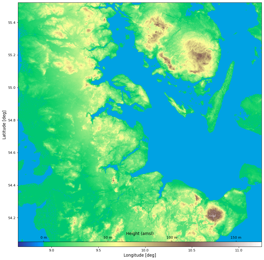
In the Height profiles section, we have already
seen, how one can query a height profile from SRTM data. It is also easy
to produce terrain maps of a region:
import matplotlib.pyplot as plt
import numpy as np
from pycraf import pathprof
from astropy import units as u

pathprof.SrtmConf.set(download='missing')

lon_t, lat_t = 9.943 * u.deg, 54.773 * u.deg  # Northern Germany
map_size_lon, map_size_lat = 1.5 * u.deg, 1.5 * u.deg
map_resolution = 3. * u.arcsec

lons, lats, heightmap = pathprof.srtm_height_map(
    lon_t, lat_t,
    map_size_lon, map_size_lat,
    map_resolution=map_resolution,
    )

_lons = lons.to(u.deg).value
_lats = lats.to(u.deg).value
_heightmap = heightmap.to(u.m).value

vmin, vmax = -20, 170
terrain_cmap, terrain_norm = pathprof.terrain_cmap_factory(
    vmin=vmin, vmax=vmax
    )
_heightmap[_heightmap < 0] = 0.51  # fix for coastal region

fig = plt.figure(figsize=(10, 10))
ax = fig.add_axes((0., 0., 1.0, 1.0))
cbax = fig.add_axes((0., 0., 1.0, .02))
cim = ax.imshow(
    _heightmap,
    origin='lower', interpolation='nearest',
    cmap=terrain_cmap, norm=terrain_norm,
    extent=(_lons[0], _lons[-1], _lats[0], _lats[-1]),
    )
cbar = fig.colorbar(
    cim, cax=cbax, orientation='horizontal'
    )
ax.set_aspect(abs(_lons[-1] - _lons[0]) / abs(_lats[-1] - _lats[0]))

ctics = np.arange(0, vmax, 50)
cbar.set_ticks(ctics)
cbar.ax.set_xticklabels(map('{:.0f} m'.format, ctics), color='k')
cbar.set_label(r'Height (amsl)', color='k')
cbax.xaxis.tick_top()
cbax.xaxis.set_label_position('top')

ax.set_xlabel('Longitude [deg]')
ax.set_ylabel('Latitude [deg]')

Here, we made use of a special matplotlib colormap, which can be produced
using terrain_cmap_factory. It returns a cmap and a
norm, which make it so that blue colors always start below a height of 0 m
(i.e., the sea level).
Note
Internally, the height-profile generation with
srtm_height_profile calls two Geodesics helper
functions provided in pycraf: geoid_inverse and
geoid_direct. They solve the “Geodesics problem” using
Vincenty’s formulae.
The underlying method is based on an iterative approach
and is used to find the distance and relative bearings between two points
(P1, and P2) on the Geoid (Earth ellipsoid), or - if P1, the bearing, and
distance are given -, it finds P2. The geodesics are the equivalent of
great-circle paths on a sphere, but on the Geoid.
Another useful feature of the Geodesics functionality is that one can query the Geographical coordinates of points at a certain distance from a central point. On the sphere, they would all be located on a circle, but on Earth it’s different:
import numpy as np
import matplotlib.pyplot as plt
from pycraf import pathprof, geometry
from astropy import units as u

lon, lat = 0 * u.deg, 70 * u.deg
bearings = np.linspace(-180, 180, 721) * u.deg
distance = 1000 * u.km

lons, lats, _ = pathprof.geoid_direct(lon, lat, bearings, distance)
ang_dist = geometry.true_angular_distance(lon, lat, lons, lats)

fig = plt.figure(figsize=(7, 6))
ax = fig.add_axes((0.1, 0.1, 0.8, 0.8))
cax = fig.add_axes((0.9, 0.1, 0.02, 0.8))
sc = ax.scatter(
    lons.to(u.deg), lats.to(u.deg),
    c=ang_dist.to(u.deg), cmap='viridis'
    )
cbar = plt.colorbar(sc, cax=cax)
cbar.set_label('Angular distance [deg]')
ax.set_xlabel('Longitude [deg]')
ax.set_ylabel('Latitude [deg]')
ax.set_aspect(1. / np.cos(np.radians(70)))
ax.grid()
Note
Make no mistake, the apparent distortion mostly comes from projecting the “sphere” to a flat projection. However, if one calculates the angular distances with the formula for the sphere, there is some deviation (from North to South). For many cases where only rough estimates are needed it will be sufficient to treat the Geoid as a normal sphere.
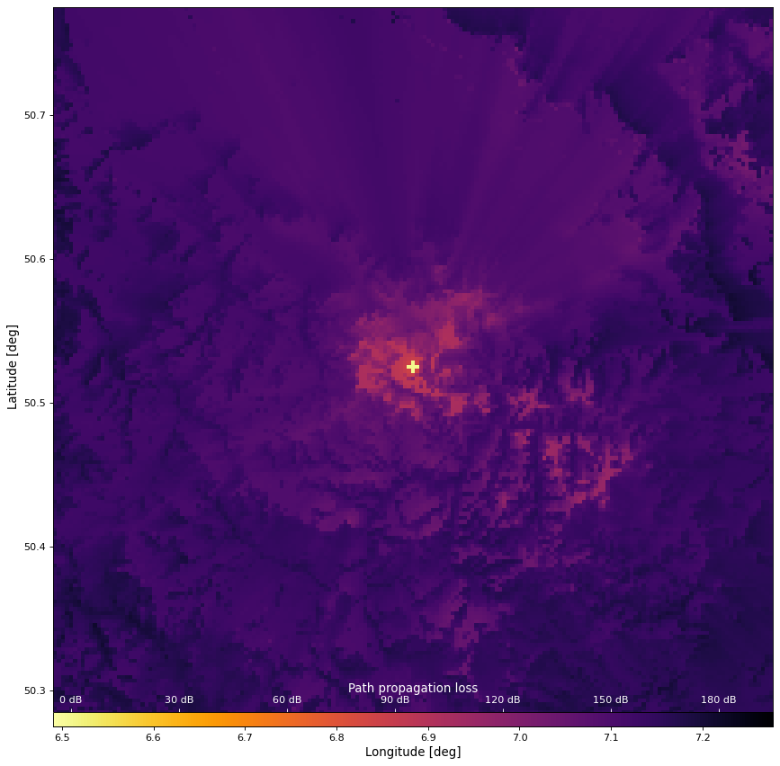
Producing maps of path propagation loss#
Often it is desired to generate maps of path attenuation values, e.g., to quickly determine regions where the necessary separations between a potential interferer and the victim terminal would be too small, potentially leading to radio frequency interference (RFI).
The simple approach would be to create a PathProp instance
for each pixel in the desired region (with the Tx being in the center of the map, and the Rx located at the other map pixels) and run the loss_complete function accordingly. This is relatively slow.
Therefore, we added a faster alternative, atten_map_fast. The idea is to generate the full height profiles only for the pixels on the map edges and re-use the arrays for the inner pixels with a clever hashing algorithm. The details of this are encapsulated in the height_map_data function, such that the user doesn’t need to understand what’s going on under the hood:
from pycraf import pathprof, conversions as cnv
from astropy import units as u


def plot_atten_map(lons, lats, total_atten):

    import numpy as np
    import matplotlib.pyplot as plt

    vmin, vmax = -5, 195
    fig = plt.figure(figsize=(10, 10))
    ax = fig.add_axes((0., 0., 1.0, 1.0))
    cbax = fig.add_axes((0., 0., 1.0, .02))
    cim = ax.imshow(
        total_atten,
        origin='lower', interpolation='nearest', cmap='inferno_r',
        vmin=vmin, vmax=vmax,
        extent=(lons[0], lons[-1], lats[0], lats[-1]),
        )
    cbar = fig.colorbar(
        cim, cax=cbax, orientation='horizontal'
        )
    ax.set_aspect(abs(lons[-1] - lons[0]) / abs(lats[-1] - lats[0]))

    ctics = np.arange(0, vmax, 30)
    cbar.set_ticks(ctics)
    cbar.ax.set_xticklabels(map('{:.0f} dB'.format, ctics), color='w')
    cbar.set_label(r'Path propagation loss', color='w')
    cbax.xaxis.tick_top()
    cbax.tick_params(axis='x', colors='w')
    cbax.xaxis.set_label_position('top')

    ax.set_xlabel('Longitude [deg]')
    ax.set_ylabel('Latitude [deg]')

    plt.show()


pathprof.SrtmConf.set(download='missing')

lon_tx, lat_tx = 6.88361 * u.deg, 50.52483 * u.deg
map_size_lon, map_size_lat = 0.5 * u.deg, 0.5 * u.deg
map_resolution = 10. * u.arcsec

freq = 1. * u.GHz
omega = 0. * u.percent  # fraction of path over sea
temperature = 290. * u.K
pressure = 1013. * u.hPa
timepercent = 2 * u.percent  # see P.452 for explanation
h_tg, h_rg = 50 * u.m, 10 * u.m
G_t, G_r = 0 * cnv.dBi, 0 * cnv.dBi
zone_t, zone_r = pathprof.CLUTTER.UNKNOWN, pathprof.CLUTTER.UNKNOWN
hprof_step = 100 * u.m

hprof_cache = pathprof.height_map_data(
    lon_tx, lat_tx,
    map_size_lon, map_size_lat,
    map_resolution=map_resolution,
    zone_t=zone_t, zone_r=zone_r,
    )  # dict-like

results = pathprof.atten_map_fast(
    freq,
    temperature,
    pressure,
    h_tg, h_rg,
    timepercent,
    hprof_cache,
    )

lons = hprof_cache['xcoords']
lats = hprof_cache['ycoords']
# index 4 is total loss without clutter/gain included:
total_atten = results['L_b'].value

plot_atten_map(lons, lats, total_atten)

For a more illustrative example, have a look at the Jupyter tutorial notebook on this topic.
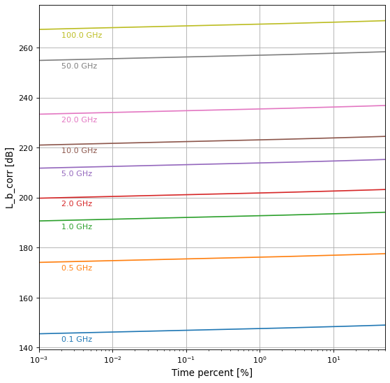
Quick analysis of a single path#
Sometimes, one needs to analyse a single path (i.e., fixed transmitter and
receiver location), which means one wants to know the propagation losses
as a function of various parameters, such as frequency, time-percentages,
or antenna heights. Depending on the number of desired samples, the approach
of creating a PathProp instance and then run one of
the loss-functions on it (see
Path attenuation) can be slow.
Therefore, another convenience function is provided,
losses_complete, which has a very similar function
signature as PathProp, but accepts ndarrays
(or rather arrays of Quantity) for most of the inputs.
Obviously, parameters such as Tx and Rx location cannot be arrays, and
as a consequence, the terrain height profile can only be a 1D array.
The following shows a typical use case (which is also contained in the Graphical user interface (pycraf-gui)):
import numpy as np
import matplotlib.pyplot as plt
from pycraf import pathprof, conversions as cnv
from astropy import units as u


lon_tx, lat_tx = 6.8836 * u.deg, 50.525 * u.deg
lon_rx, lat_rx = 7.3334 * u.deg, 50.635 * u.deg
hprof_step = 100 * u.m  # resolution of height profile
omega = 0. * u.percent
temperature = 290. * u.K
pressure = 1013. * u.hPa
h_tg, h_rg = 5 * u.m, 50 * u.m
G_t, G_r = 0 * cnv.dBi, 15 * cnv.dBi
zone_t, zone_r = pathprof.CLUTTER.URBAN, pathprof.CLUTTER.SUBURBAN

frequency = np.array([0.1, 0.5, 1, 2, 5, 10, 20, 50, 100])
time_percent = np.logspace(-3, np.log10(50), 100)

# as frequency and time_percent are arrays, we need to add
# new axes to allow proper broadcasting
results = pathprof.losses_complete(
    frequency[:, np.newaxis] * u.GHz,
    temperature,
    pressure,
    lon_tx, lat_tx,
    lon_rx, lat_rx,
    h_tg, h_rg,
    hprof_step,
    time_percent[np.newaxis] * u.percent,
    zone_t=zone_t, zone_r=zone_r,
    )

fig, ax = plt.subplots(1, figsize=(8, 8))
L_b_corr = results['L_b_corr'].value
t = time_percent.squeeze()
lidx = np.argmin(np.abs(t - 2e-3))
for idx, f in enumerate(frequency.squeeze()):
    p = ax.semilogx(t, L_b_corr[idx], '-')
    ax.text(
        2e-3, L_b_corr[idx][lidx] - 1,
        '{:.1f} GHz'.format(f),
        ha='left', va='top', color=p[0].get_color(),
        )

ax.grid()
ax.set_xlim((time_percent[0], time_percent[-1]))
ax.set_xlabel('Time percent [%]')
ax.set_ylabel('L_b_corr [dB]')
Note
Even with the Tx/Rx location and the terrain height profile being constant
for one call of the losses_complete function, the
computing time can be substantial. This is because changes in the
parameters frequency, h_tg, h_rg, version, zone_t, and zone_r
have influence on the propagation path geometry. In the broadcasted
arrays,
the axes associated with the mentioned parameters should vary as slow as
possible. The underlying implementation will trigger a re-computation of
the path geometry if one of these parameters changes. Therefore, if the
broadcast axes for frequency and time_percent would have been chosen
in the opposite manner, the function would run about an order of magnitude
slower!
See Also#
Astropy Units and Quantities package, which is used extensively in pycraf.
Reference/API#
pycraf.pathprof Package#
Contains functions to construct height profiles and terrain maps from SRTM data, calculate shortest path on the Geoid - so-called geodesics -, and perform path propagation/attenuation estimation.
Functions#
|
Calculate power output level after UE power control. |
|
Calculate annual equivalent time percentage, p, from worst-month time percentage, p_w, according to ITU-R P.452-16 Eq (1). |
|
Calculate attenuation maps using a fast method. |
|
Calculate attenuation along a path using a parallelized method. |
|
Calculate building entry loss (BEL). |
|
Calculate the Clutter loss of a propagating radio wave according to ITU-R P.452-16 Eq (57). |
|
Calculate the Clutter loss according to IMT.CLUTTER document (method 2). |
|
Query delta_N and N_0 values from digitized maps by means of bilinear interpolation. |
Calculate effective Earth radius exceeded for beta_0 percent of time, a_beta, according to ITU-R P.452-16 Eq (6b). |
|
Calculate effective Earth radius factor exceeded for beta_0 percent of time, k_beta, according to ITU-R P.452-16. |
|
|
Calculate median effective Earth radius factor, k_50, according to ITU-R P.452-16 Eq (5). |
|
Calculate median effective Earth radius, a_e, according to ITU-R P.452-16 Eq (6a). |
|
Calculate WGS84 surface area over interval [lon1, lon2] and [lat1, lat2]. |
|
Solve direct Geodesics problem using Vincenty's formulae. |
|
Solve inverse Geodesics problem using Vincenty's formulae. |
|
Calculate height profiles and auxillary maps needed for |
|
Calculate height profile auxillary data needed for |
|
Calculate height profile auxillary data needed for |
|
Calculate los/non-los propagation losses Rural-Macro IMT scenario. |
|
Calculate los/non-los propagation losses Rural-Macro IMT scenario. |
|
Calculate los/non-los propagation losses Rural-Macro IMT scenario. |
Convert a map of landcover class IDs to P.452 clutter types. |
|
|
Calculate the total loss of a propagating radio wave according to ITU-R P.452-16 Eq (58-64). |
|
Calculate the Diffraction loss of a propagating radio wave according to ITU-R P.452-16 Eq (14-44). |
|
Calculate the ducting/layer reflection loss, L_ba, of a propagating radio wave according to ITU-R P.452-16 Eq (46-56). |
|
Calculate the free-space loss, L_bfsg, of a propagating radio wave according to ITU-R P.452-16 Eq (8-12). |
|
Calculate the tropospheric scatter loss, L_bs, of a propagating radio wave according to ITU-R P.452-16 Eq (45). |
|
Calculate propagation losses for a fixed path using a parallelized method. |
|
Produce kmz file for use in GIS software (e.g., Google Earth). |
|
Calculate delta_N, beta_0, and N_0 values from digitized maps, according to ITU-R P.452-16 Eq (2-4). |
|
Retrieve interpolated GeoTiff raster values for given WGS84 coordinates (longitude, latitude). |
|
Change maximum number of threads to use. |
|
Interpolated SRTM terrain data extracted from ".hgt" files. |
|
Extract terrain map from SRTM data. |
|
Extract a height profile from SRTM data. |
|
Produce terrain colormap and norm to be used in plt.imshow. |
|
Convert WGS84 (longitude, latitude) to pixel space of a GeoTiff. |
Classes#
|
|
|
|
|
Container class that holds all path profile properties. |
|
Provide a global state to adjust SRTM configuration. |
Variables#
Effective Earth radius for beta_0 percent |
|
Built-in mutable sequence. |
|
Effective Earth radius factor for beta_0 percent |
|
Earth Radius |
|
Available clutter types in Rec. ITU-R P.452-16#
Value |
Alias |
\(h_\mathrm{a}~[\mathrm{m}]\) |
\(d_\mathrm{k}~[\mathrm{m}]\) |
|---|---|---|---|
-1 |
CLUTTER.UNKNOWN |
0 |
0 |
0 |
CLUTTER.SPARSE |
4 |
100 |
1 |
CLUTTER.VILLAGE |
5 |
70 |
2 |
CLUTTER.DECIDIOUS_TREES |
15 |
50 |
3 |
CLUTTER.CONIFEROUS_TREES |
20 |
50 |
4 |
CLUTTER.TROPICAL_FOREST |
20 |
30 |
5 |
CLUTTER.SUBURBAN |
9 |
25 |
6 |
CLUTTER.DENSE_SUBURBAN |
12 |
20 |
7 |
CLUTTER.URBAN |
20 |
20 |
8 |
CLUTTER.DENSE_URBAN |
25 |
20 |
9 |
CLUTTER.HIGH_URBAN |
35 |
20 |
10 |
CLUTTER.INDUSTRIAL_ZONE |
20 |
50 |
Conversion between Landcover classes and P.452 clutter types#
The following tables provide a mapping between Corine and IGBP Landcover classes and P.452 clutter types. It is based on common sense, but unofficial! Note, that ITU-R also provides clutter information in its ITU Digitized World Map (IDWM) and Subroutine Library (32-bit) but it’s available for (old versions of) Windows, only, and comes with a steep price tag.
Corine ID |
Explanation |
P.452 Class |
|---|---|---|
111 |
Continuous urban fabric |
URBAN |
112 |
Discontinuous urban fabric |
SUBURBAN |
121 |
Industrial or commercial units |
INDUSTRIAL_ZONE |
122 |
Road and rail networks and associated land |
INDUSTRIAL_ZONE |
123 |
Port areas |
INDUSTRIAL_ZONE |
124 |
Airports |
INDUSTRIAL_ZONE |
131 |
Mineral extraction sites |
INDUSTRIAL_ZONE |
132 |
Dump sites |
INDUSTRIAL_ZONE |
133 |
Construction sites |
INDUSTRIAL_ZONE |
141 |
Green urban areas |
URBAN |
142 |
Sport and leisure facilities |
INDUSTRIAL_ZONE |
211 |
Non-irrigated arable land |
SPARSE |
212 |
Permanently irrigated land |
SPARSE |
213 |
Rice fields |
SPARSE |
221 |
Vineyards |
SPARSE |
222 |
Fruit trees and berry plantations |
SPARSE |
223 |
Olive groves |
SPARSE |
231 |
Pastures |
SPARSE |
241 |
Annual crops associated with permanent crops |
SPARSE |
242 |
Complex cultivation patterns |
SPARSE |
243 |
Land principally occupied by agriculture |
SPARSE |
244 |
Agro-forestry areas |
SPARSE |
311 |
Broad-leaved forest |
DECIDIOUS_TREES |
312 |
Coniferous forest |
CONIFEROUS_TREES |
313 |
Mixed forest |
DECIDIOUS_TREES |
321 |
Natural grasslands |
SPARSE |
322 |
Moors and heathland |
SPARSE |
323 |
Sclerophyllous vegetation |
SPARSE |
324 |
Transitional woodland-shrub |
SPARSE |
331 |
Beaches, dunes, sands |
SPARSE |
332 |
Bare rocks |
SPARSE |
333 |
Sparsely vegetated areas |
SPARSE |
334 |
Burnt areas |
SPARSE |
335 |
Glaciers and perpetual snow |
SPARSE |
411 |
Inland marshes |
UNKNOWN |
412 |
Peat bogs |
UNKNOWN |
421 |
Salt marshes |
UNKNOWN |
422 |
Salines |
UNKNOWN |
423 |
Intertidal flats |
UNKNOWN |
511 |
Water courses |
UNKNOWN |
512 |
Water bodies |
UNKNOWN |
521 |
Coastal lagoons |
UNKNOWN |
522 |
Estuaries |
UNKNOWN |
523 |
Sea and ocean |
UNKNOWN |
IGBP ID |
Explanation |
P.452 Class |
|---|---|---|
1 |
Evergreen needleleaf forests |
CONIFEROUS_TREES |
2 |
Evergreen broadleaf forests |
DECIDIOUS_TREES |
3 |
Deciduous needleleaf forests |
CONIFEROUS_TREES |
4 |
Deciduous broadleaf forests |
DECIDIOUS_TREES |
5 |
Mixed forests |
DECIDIOUS_TREES |
6 |
Closed shrublands |
SPARSE |
7 |
Open shrublands |
SPARSE |
8 |
Woody savannas |
DECIDIOUS_TREES |
9 |
Savannas |
SPARSE |
10 |
Grasslands |
SPARSE |
11 |
Permanent wetlands |
SPARSE |
12 |
Croplands |
SPARSE |
13 |
Urban and built-up lands |
URBAN |
14 |
Cropland/natural vegetation mosaics |
SPARSE |
15 |
Snow and ice |
UNKNOWN |
16 |
Barren |
UNKNOWN |
17 |
Water bodies |
UNKNOWN |